Quickstart

Take a small-scale nonlinear New Keynesian model with ZLB as a starting point, which is provided as an example (find the yaml file here). Here is how to simulate it and plot nonlinear impulse responses. Start with some misc imports and load the package:

import matplotlib.pyplot as plt
import econpizza as ep

# only necessary if you run this in a jupyter notebook:
%matplotlib inline

Next, load the model and solve for the steady state.

# the path to the example YAML
example_nk = ep.examples.nk

# load the NK model
mod = ep.load(example_nk)
_ = mod.solve_stst()

(load:) Parsing done.
    Iteration   1 | max. error 7.89e-01 | lapsed 0.2448
    Iteration   2 | max. error 5.07e-01 | lapsed 0.2935
(solve_stst:) Steady state found (0.38772s). The solution converged.

Finally, set a 4% discount factor shock and simulate it:

# shock the discount factor by 4%
shk = ('e_beta', .04)

# find the nonlinear trajectory
x, flag = mod.find_path(shock=shk)

    Iteration   1 | max error 1.71e-01 | lapsed 0.4717s
    Iteration   2 | max error 3.89e-01 | lapsed 0.4734s
    Iteration   3 | max error 2.35e-01 | lapsed 0.4746s
    Iteration   4 | max error 2.50e-01 | lapsed 0.4758s
    Iteration   5 | max error 6.81e-02 | lapsed 0.4769s
    Iteration   6 | max error 2.14e-02 | lapsed 0.4779s
    Iteration   7 | max error 5.58e-06 | lapsed 0.4790s
    Iteration   8 | max error 3.98e-12 | lapsed 0.4802s
(find_path:) Stacking done (0.568s). The solution converged.

The rest is plotting…

# plotting
fig, axs = plt.subplots(2,2)
for i,v in enumerate(('y', 'pi', 'r', 'beta')):

    axs.flatten()[i].plot(x[:35,mod.var_names.index(v)])
    axs.flatten()[i].set_xlabel(v)

fig.tight_layout()

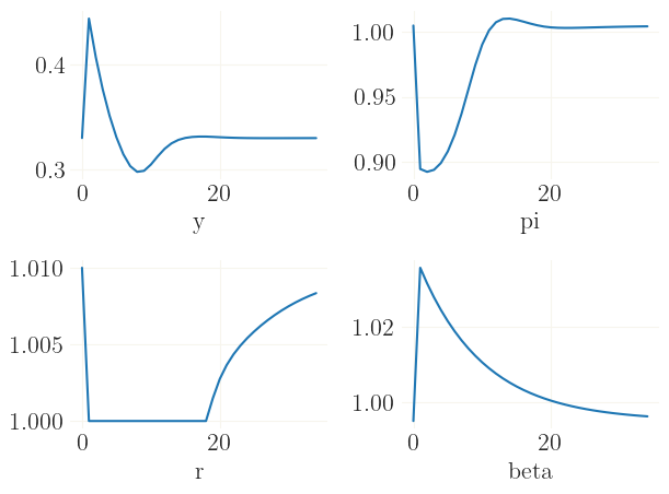
The impulse responses are the usual dynamics of a nonlinear DSGE model with the zero-lower bound on nominal interest rates.

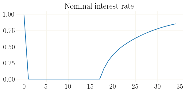
Alternatively to specifying a shock, you can instead provide the initial conditions:

# use the jax implementation of numpy
import jax.numpy as jnp

# get the steady state as initial condion
x0 = mod['stst'].copy()
# and emulate again a 4% shock
x0['beta'] *= 1.04

# solving...
x, flag = mod.find_path(init_state=x0.values())

# plotting...
plt.figure(figsize=(7,3))
plt.plot(100*jnp.log(x[:35,mod.var_names.index('r')]))
plt.title('Nominal interest rate')

    Iteration   1 | max error 1.51e-01 | lapsed 0.0016s
    Iteration   2 | max error 2.92e-01 | lapsed 0.0031s
    Iteration   3 | max error 1.57e-01 | lapsed 0.0042s
    Iteration   4 | max error 3.66e-02 | lapsed 0.0054s
    Iteration   5 | max error 3.93e-03 | lapsed 0.0065s
    Iteration   6 | max error 3.90e-05 | lapsed 0.0077s
    Iteration   7 | max error 5.68e-10 | lapsed 0.0088s
(find_path:) Stacking done (0.122s). The solution converged.

Text(0.5, 1.0, 'Nominal interest rate')